Math Topics for Quant Interviews
Do you know the difference in meaning between “stochastic” and “statistic”? Does Black-Scholes (BS) stand for “Boring Stuff” in your mind? Does the thought of explaining how to calculate an R-squared value make you wish you had reviewed your econometrics textbook before arriving at your interview?
Most Hedge Funds that are looking for Quants will not expect you to have strong knowledge of finance developed yet, unless you’ve worked in the field before. Nonetheless, there are some basic concepts you should be familiar with; even if you haven’t taken a finance class; we have detailed those below. Knowing some elementary financial concepts shows an initiative to get yourself up to speed in your desired industry.
Mathematical Finance Topics
What is Black-Scholes (B-S)? Walk me through the derivation.
B-S is a mathematical formula that is used to determine the price of a European call option (or European put option) on a financial instrument. The model assumes that asset price movements follow geometric Brownian motion with constant drift and volatility. Brownian motion originally referred to the microscopic motions of a small particle floating in a liquid; if stock prices move in a similar way, then the random increments or price changes will be normally distributed with an infinitesimal variance.
Assume that the asset price S follows the following process:
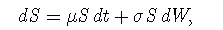
where μ and σ are constant, t stands for time, and W is a Wiener process. (A Wiener process is a type of stochastic process with a mean change of zero and a variance equal to Δt—this is simply another way to describe Brownian motion. If the value of a variable following a Wiener process is x0 at time zero, at time T, it will be normally distributed with mean = x0 and a standard deviation equal to the square root of T.)
The basis of Black-Scholes is Ito’s Lemma, which explains the process of stochastic behavior. If a variable x follows an Ito process (dx = a(x, t) + b(x, t)dW) then Ito’s Lemma shows that a function G, of x and t, follows the process:
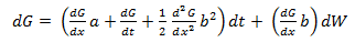
If f is the price of a call option on stock S, and f is a function of S and t, then via Ito’s Lemma:

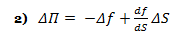
The above formula is key to the derivation of the B-S equation, which incorporates the constant price variation (volatility) of the stock, the time value of money, the option’s strike price and the option’s time to expiry. Black-Scholes for a non-dividend paying stock depends on the construction of a riskless portfolio, where positions are taken in bonds (cash), the underlying stock and options. If one holds –1 units (i.e., sold short one unit) of a derivative f plus df/ds shares, the change in the value of this portfolio Π over time Δt is equal to:
If the stock price can be modeled as above:
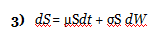
then via Ito’s Lemma 1) and 3) above:
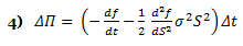
Notice how the above equation (the change in the portfolio value) does not involve dW. During time increment Δt, the portfolio is not subject to random movement—it must earn the riskless rate. Because
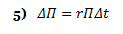
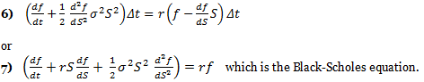
using 2) and 4) in conjunction with 5) above yields:
What are the assumptions made in Black-Scholes?
- There is no arbitrage opportunity (i.e., there is no way to make a riskless profit).
- It is possible to borrow and lend cash at the same constant risk-free interest rate.
- It is possible to buy and sell stocks in any amount (including fractional amounts); there is no restraint on short selling.
- There are no transaction costs (the market is frictionless).
- Stock prices follow geometric Brownian motion with constant drift and constant volatility.
- Note: The original B-S equation assumed no dividend payments. However, dividends can be taken into account by subtracting them from the risk-free rate, assuming that both the dividend and the risk-free rate are continuously compounding.
What are the “Greeks” in Black-Scholes? What are Vanna and Volga?
The “Greeks” are the model outputs from Black-Scholes, known as Greeks due to their mathematical notation with Greek letters. They provide information about the sensitivity of outputs of the model to changes in the inputs into the model.
- Delta: Measures the rate of change in the option value with respect to changes in the underlying asset’s price (the first derivative of the option price with respect to the underlying price). It loosely equals the probability that the option finishes in-the-money. Delta for a call ranges from 0 to 1, and from -1 to 0 for puts.
- Gamma: Measures the rate of change of the option delta with respect to the change in the underlying asset price (the second derivative of the option price with respect to the underlying price). Even if the underlying asset price remains unchanged, the option delta for an in-the-money option increases as expiration nears; the opposite is true for an out-of-the-money option. The gamma of an option indicates how the delta of an option will change for a one-point move in the underlying asset. In other words, the Gamma shows the option delta’s sensitivity to market price changes. Gamma is important for maintaining a delta neutral position.
- Vega: Measures the sensitivity of the option to changes in implied volatility. It equals the first derivative of the option price with respect to the volatility of the underlying asset. Vega is typically expressed as the amount of money per underlying share that the option’s value will gain or lose as volatility rises or falls by 1%. Vega is most sensitive when the option is at-the-money and tapers off either side as the market trades above/below the strike. Some option trading strategies that are particularly Vega-sensitive are straddles, where a profit can be made when volatility increases or decreases without a move in the underlying asset. Vega falls as an option moves to become in-the-money or out-of-the money.
- Theta: Theta measures how fast the premium of an option decays with time or how much value an option’s price will diminish per day—including non-business days (all other factors being constant). Note that it is not possible to hedge the passage of time. The nearer the expiration date, the higher the Theta. Option trading strategies that are particularly Theta-sensitive include Calendar Spreads, where traders maintain a net positive Theta by buying longer-dated options and selling shorter-dated options, profiting when the underlying stock remains within a tight range.
- Rho: Rho measures the sensitivity of a stock option’s price to a change in interest rates; typically, changes in interest rates over short time periods have very little effect on options where the underlying asset is not rate sensitive (equities instead of bonds, for example). Call options rise in value when interest rates rise; the opposite is true for puts. Rho increases as time to expiration becomes longer.
- Extra Credit: Vanna and Volga: Vanna is the sensitivity of the option delta with respect to a change in volatility, and can be helpful in maintaining a Delta-hedged or Vega-hedged portfolio. Volga (sometimes known as Vomma) is the second derivative of the option value with respect to a change in volatility; in other words, it measures the rate of change in Vega as volatility changes. When Volga is positive, a position will become long Vega as implied volatility increases. An initially Vega-neutral, long-Volga position can be constructed from ratios of options at different strikes.
What is delta hedging? Are there scenarios where it’s not profitable?
Delta hedging is the process of setting or keeping the delta of a portfolio consisting of assets and options on those assets as close to zero as possible, typically by buying or selling some amount of the asset such that the total exposure from the asset plus the option equals zero. Generally speaking, when one purchases options and delta hedges, one wants future realized volatility to be higher than the implied volatility at which the option was purchased.
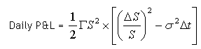
When a position is delta-hedged, the daily P&L on a delta-hedged option position equals:
where “Other” includes the P&L from financing the underlying position as well as P&L due to changes in interest rates and dividend expectations.
Rewritten formulaically,
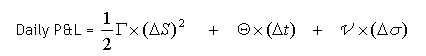
where ΔS is the change in the underlying stock price, Δt is the fraction of time elapsed, Δσ is the change in implied volatility, and Γ, Θ, and ν refer to Gamma, Theta and Vega, respectively.
Typically, an investor who sells options (and is short gamma) and is delta hedging should make money if future realized volatility is lower than the volatility that the option was priced with (its implied volatility). So what’s going on? If implied volatility is constant and interest rates are assumed to equal zero, then
So that:
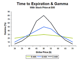
The second half of the above equation reflects the difference between an asset’s 1-day squared return (its variance) and the 1-day implied variance. When the difference between these two variances equals zero, the daily P&L equals zero as well. However, the Gamma (Γ) of an option does not remain constant through time or through asset price moves. Gamma reaches its maximum value (at a given time) when an option is at-the-money. (However, if overall volatility is high, gamma tends to be stable across all strike prices, as the time value of deeply in/out-of-the-money options is already quite substantial.) For a given price, Gamma increases as the time to expiry decreases.
While over the lifetime of an option, a trader who is short Gamma may find that realized volatility is below the implied volatility over which the option was sold, the P&L of a delta-hedged portfolio is path-dependent.
A short option holder who is Delta hedging may be “up” in P&L during the early period of the trade, only to lose money at the very end when asset prices oscillate around the strike in the final months, causing Gamma to rise. If realized volatility remained low, higher Gamma would be a good thing, but an environment of rising volatility in tandem with higher Gamma will lead to losses. Because the daily P&L of the option position was weighted by a volatility spread that was negative (realized > implied), the final P&L “drowned,” even though the realized volatility over the entire history of the option was below its initial implied level.
What is realized volatility and how is it calculated?
Realized volatility is the historical annualized standard deviation of an asset’s log returns. It is calculated by 1) taking the standard deviation of the log returns of an asset and 2) multiplying this value by the square root of the frequency of the data.
For example, with weekly stock prices:
|
Stock Price
|
Log Return
|
Log Return (decimals)
|
|
| Week 1 |
100
|
||
| Week 2 |
107
|
ln(107/100)
|
0.06766
|
| Week 3 |
92
|
ln(92/107)
|
–0.15104
|
| Week 4 |
88
|
ln(88/92)
|
–0.04445
|
|
Std Deviation
|
0.10936
|
Frequency of data: Weekly, or 52 weeks in a year.
The volatility of the above data set = (Std Deviation of log returns) × Sqrt(52)
Note: With daily price data, it is assumed that there are 252 trading (or business) days in a year, so that the frequency adjustment would be Sqrt(252).
How is realized volatility different from implied volatility?
Realized volatility is based entirely on an asset price’s past behavior over some calculated period; implied volatility is an input into the Black-Scholes model that is based on an asset’s assumed volatility over the option period. Note that future volatility may or may not resemble past volatility.
How much should I pay for an option when the future volatility of the underlying is zero?
When the implied volatility of an asset is zero, the future price is known with certainty—there is not a distribution around a mean value. Based on the ability to replicate the payoff of an asset risklessly using cash and options, under the risk-neutral measure of Black-Scholes, the asset is expected to grow exactly at the risk-free rate for the period; one may take this future value, subtract the exercise (strike) price, and discount the future gain to the present value using the same risk-free rate.
What is a variance swap?
A variance swap is an instrument that allows investors to trade future realized (or historical) volatility against current implied volatility. Only variance—the square of volatility—can be replicated with a static hedge. The final payment = Variance Notional Amount × (Final Realized Volatility2 – Strike Price2). Unlike the delta-hedged example above, a long variance position will always benefit when realized volatility is higher than implied at inception, and conversely for a short position.
How is a forward FX rate calculated?
An exchange rate is a ratio: the price of one country’s currency expressed in another country’s currency. Unlike equities, where all equity prices worldwide can decline, this is not true for the currencies; if the dollar has depreciated against the pound, then the pound by definition will have strengthened (or appreciated) against the dollar.
A forward FX rate is an arbitrage free rate at a future point in time T that takes into account the riskless rate of return that can be earned in each country in local currency over the interval T. For example: If today’s exchange rate is 100 units of foreign currency per 1 USD, and 1-year interest rates are 10% abroad and 5% in the U.S., then one would have either $1.05 in the U.S. after one year or 110 foreign currency units after one year. In order to avoid a situation where one could earn riskless profits, the 1-year forward exchange rate will equal 110 foreign currency units per $1.05, or 104.76 units of foreign currency per 1 USD. In this case, an investor would be indifferent between borrowing in foreign currency at today’s spot rate and earning a higher interest rate abroad, since the rate at which he can contractually exchange the foreign currency for his home currency is lower by the ratio of the current interest rate differential.
What is the difference between a forward contract and a futures contract? Under what cases are the prices of the two contracts the same?
A forward contract is an agreement between two parties, in which a buyer agrees to buy a quantity of an asset at a specific price from the seller at a future date. In a forward transaction, no actual cash changes hands. Forward contracts are traded over-the-counter (OTC), i.e., not on an exchange. Both the buyer and seller are bound by the contractual terms, where the price remains fixed. Because a forward is not exchange-traded, there may be a lack of liquidity; moreover, each party is subject to non-performance by the other—either buyer or seller may fail to honor her end of the contract.
A futures contract is an agreement to buy or sell an asset at a certain time in the future (the delivery date) at a pre-set price. The future date is called the delivery date or final settlement date. The pre-set price is called the futures price. The price of the underlying asset on the delivery date is called the settlement price. The futures price converges towards the settlement price (or future spot price) on the delivery date. Terms are standardized, rather than customized. Futures are traded on organized exchanges, and use a clearing house to provide protection against non-performance to both the buyer and the seller. The price of the futures contract can change prior to delivery; in order to guarantee that neither party defaults on the obligation, both participants must settle daily price changes as per the contract values (daily margin) in addition to posting an initial margin.
There is a difference between forward and futures prices when interest rates are stochastic—in other words, when they vary unpredictably over time. If an asset is positively correlated with interest rates, then the holder of a long futures contract will profit if the asset price rises—both from the fact that the direction of the market move is positive for the long futures holder, but also because the daily margin posted from the market move can be invested at a higher rate than the prior day’s rate. When asset prices are correlated with interest rates, futures prices will typically be higher than forward prices.
Statistics
What is a lognormal distribution?
A lognormal distribution is a distribution of values that are positively skewed (versus the symmetric distribution of a normal distribution). In a lognormal distribution, values may not go below zero but can have unlimited positive potential. Variables that are distributed lognormally include stock prices and (typically) interest rates.
What is a correlation coefficient? How is it calculated?
A correlation coefficient is a measure of the interdependence of two random variables and ranges in value from –1 to +1, indicating perfect negative correlation at –1, absence of correlation at zero, and perfect positive correlation at +1. It is calculated as the covariance of the two variables, divided by the square root of the product of each variable’s variance (i.e., the product of each variable’s standard deviation). Note that an equity Beta for stock x is the covariance of the stock x with the market divided by the variance of the market.
What is the difference between a permutation and combination?
If order does matter, compute occurrences using the formula for a permutation (permutation = position). If the order doesn’t matter, use the formula for a combination.
When items may only be selected once (i.e., there is no repetition) and the order of selection matters, the number of possible outcomes equals: n! ÷ (n – r)! where n is the number of items to choose from, and r items are chosen. This is a permutation.
When items may only be selected once (i.e., there is no repetition) and the order of selection doesn’t matter, the number of possible outcomes equals: n! ÷ [r! × (n – r)!] where n is the number of items to choose from, and r items are chosen. This combination is typically written using the following shorthand: nCr. Combinations are symmetric, so choosing 3 balls out of 16 or choosing 13 balls out of 16 results in the same number of combinations.
What is the probability that I flip this penny 5 times, it will come up heads at least 2 times?
The trick here is the phrase “at least 2.” This means: what is the probability that of 5 flips, I will end up with 2 or 3 or 4 or 5 heads? Think of this as the inverse to the problem: what is the probability that of 5 flips, I see a head only once or no times at all?
The probability out of 5 flips of getting 0 heads:
= (probability of getting 5 tails)
= (0.5)5
= 3.125%
The probability out of 5 flips of getting 1 head:
=(probability of getting 4 tails) × (probability of getting 1 head) × 5C1
= (0.5)4 × (0.5)1 × 5C1
= (0.5)4 × (0.5)1 × 5! ÷ (1! × 4!)
= 15.625%
The probability of getting 0 or 1 heads in 5 flips = 3.125% + 15.625% = 18.750%.
The probability of getting 2 or more heads in 5 flips = 1 – 18.75% = 81.25%.
What is a Monte Carlo simulation?
A Monte Carlo simulation is a computerized mathematical procedure for sampling random outcomes for a given process. It provides a range of possible outcomes (and their associated probabilities) rather than a discrete point estimate of a given outcome. Monte Carlo simulation performs risk analysis by building models of possible results by substituting a range of values—a probability distribution—for any factor that has inherent uncertainty. It calculates results over and over, each time using a different set of random values chosen from the probability functions. During a Monte Carlo simulation, values are sampled at random from the input probability distributions. Each set of results from that sample is recorded; the values comprise a probability distribution of possible outcomes. Depending upon the number of uncertainties and the ranges specified for them, a Monte Carlo simulation could involve thousands or tens of thousands of recalculations.
Monte Carlo simulation provides a number of advantages over deterministic, or “single-point estimate” analysis:
1) Probabilistic Results. Results show not only what could happen, but also how likely each outcome is.
2) Sensitivity Analysis. In a Monte Carlo simulation, it’s easy to see which inputs had the biggest effect on line results. In deterministic models, it’s difficult to model different combinations of values for different inputs to see the effects of truly different scenarios.
3) Correlation of Inputs. In a Monte Carlo simulation, it’s possible to model relationships among input variables.
Monty Hall problem: Assume that I tell you that a prize is behind one of three doors. If you pick a door (say Door #2), and I tell you that the prize is not behind another door (Door #3, for example), and I give you the option of remaining with your first pick (Door #2) versus switching to Door #1, should you switch? Why?
This question has been asked for decades; the answer is much simpler than many think. The probability that a prize is behind Door 1 is 1/3; the probability that the prize is behind Door 2 is 1/3; and similarly, the probability that the prize is behind Door 3 is 1/3.
Before any additional information is given, the key is that the probability that the prize is behind Door 1 OR Door 3 is 1/3 + 1/3 = 2/3. If I then tell you that the prize is NOT behind Door 3, then the probability that the prize is behind Door 1 is now 2/3 (since I’ve just told you that there is a 0% probability that the prize is behind Door 3).
If the probability that the prize is behind Door 2 is 1/3, but the probability that the prize is behind Door 1 is now 2/3 (with the new information that the prize is NOT behind Door 3), then you should switch your choice of doors to Door 1; switching from Door 2 to Door 1 doubles your chance of winning (raises the probability from 1/3 to 2/3).
Birthday problem: What’s the probability that in a room full of k people, at least 2 people will have the same birthday?
Each person has 365 “possible” birthdays (ignoring leap years); in a room of k people, the total number of possible birthdays is 365k.
In order for at least 2 people to have the same birthday, this means that 2 or 3 or 4….have the same birthday, which is the “inverse” or complement of none of the k birthdays in the group being the same. This latter event is a permutation; if John is born on January 1 and Jeff is born on December 31, this is a different outcome than John being born on December 31 and Jeff being born on January 1 (i.e., position matters.) The total number of ways to choose k different birthdays from 365 elements (with no repetitions) is 365! ÷ (365 – k)!. So for a room full of k people, the probability that at least 2 have the same birthday is:
1 – [365! ÷ (365 – k)!] ÷ 365k
When k = 15, the probability is 25.3%; when k = 50, the probability rises to 97.0%!
What is Bayes’ Theorem and when is it used?
Bayes’ theorem gives the relationship between the probabilities of Event A and Event B, and the conditional probability of Event A occurring given the occurrence of Event B, written P (A|B).
For example, assume a drug test is correct 99% of the time, meaning that when someone has used the drug, they test positive for the drug 99% of the time; when someone hasn’t used the drug, they test negative 99% of the time. If 2% of the population uses the drug, what is the probability that someone who has tested positive actually does use the drug?
Prob(drug user) = 2%
Prob(test positive | drug user) = 99%
Prob(test positive | not drug user) = 1%
So we have:
Prob(drug user |test positive) =
[Prob(test positive |drug user) × Prob(drug user)] ÷ {[Prob(test positive |drug user) × Prob(drug user)] + [Prob (test positive |not drug user) × Prob(not drug user)]}
Therefore:
Prob(drug user |test positive) = [99% × 2%] / [(99% × 2%) + (1% × 98%)] = 66.9%
So for a positive test, there’s only a 2/3 chance that the test-taker is a drug user.
Econometrics
What is an R2 statistic?
An R2 statistic is a measure of goodness-of-fit, also known as the coefficient of determination. It is the proportion of variability in a data set that is accounted for by the chosen model. In a simple linear regression (y = mx + b), the R2 statistic is the percentage of variability in ‘y’ that can be explained by movements in ‘x.’ Note that in a linear regression, R2 equals the square of the sample correlation coefficient between the outcomes (y) and their predicted values, and can be thought of as a percentage from 1 to 100.
What is a random walk? Is it stationary or non-stationary?
A random walk is a path that consists of taking successive random steps. Often, the “steps” taken by a stock price are assumed to follow a random walk. Random walks are not stationary, i.e., where you “are” in the walk depends on where you were immediately prior to your last step. Non-stationary behaviors can include trends, cycles, random walks or combinations of the three. Note that while non-stationary data cannot be modeled or forecasted, the data can usually be transformed so that they can be modeled.
In a pure random walk (Yt = Yt-1 + εt), the value or location at time t will be equal to the last period value plus a stochastic (non-systematic) component that is a white noise, which means εt is independent and identically distributed with mean of 0 and variance equal to σ². The random walk is a non-mean reverting process that can move away from the mean either in a positive or negative direction. Put another way, the means, variances and co-variances of the walk change over time. Another characteristic of a random walk is that the variance evolves over time and goes to infinity as time goes to infinity; therefore, a random walk cannot be predicted.
What happens if you create a regression based on 2 variables that each are continuously increasing with time?
If you attempt to model two series that are both time-dependent (say, consumption and income), you will get a spurious regression, i.e., a model with a high R2, but poor predictive properties. This is because both series are non-stationary. With non-stationary variables, one needs to transform them into stationary series; the easiest way to do this is by differencing, or looking at changes in the series. Changes in a non-stationary series are usually stationary.
What to do if two series are non-stationary: Rather than differencing each series, one may be able to create a better model by finding a cointegrating relationship. With cointegration, the aim is to detect any common stochastic trends in the underlying data; whereas the two series may not be stationary, the difference between two non-stationary series may itself, be stationary.
If I have a regression between x and y, what test statistics should I look at to determine whether I have a good model?
- R2: See above. Explains how much of the movement in the independent variable can be explained by the dependent variables chosen.
- t-Statistic: In a least squares regression, the t-statistic is the estimated regression coefficient of a given independent variable divided by its standard error. If the t-statistic is more than 2 (i.e., the coefficient is at least twice as large as the standard error), one can conclude that the variable in question has a significant impact on the dependent variable.
- F-Test: In a regression model, the F-test allows one to compare the null hypothesis.
- H0: All non-constant coefficients in the regression equation are zero (i.e., the model has no explanatory power).
- Ha: At least one of the non-constant coefficients in the regression equation is non-zero.
The F-test tests the joint explanatory power of the variables, while the t tests test their explanatory power individually. One rejects the null hypothesis when the F statistic is greater than its critical value.
- Durbin-Watson statistic: the Durbin–Watson (d) statistic measures the presence of autocorrelation in the residuals. The value of d always lies between 0 and 4. A value of 2 indicates no autocorrelation. If the Durbin–Watson statistic is substantially less than 2, there is evidence of positive serial correlation.
- Akaike Information Criterion: From among a set of models, the Akaike Information Criterion (AIC) suggests the preferred model as the one with the minimum AIC value. The AIC = 2k – 2 × ln(L) where k is the number of parameters in the statistical model, and L is the maximized value of the likelihood function for the estimated model. The AIC rewards goodness of fit, but also includes a penalty that is an increasing function of the number of estimated parameters, which discourages overfitting.
If I have data from 1912-2012, what’s the danger if I build a model forecasting values in 2012 using all of the historical data?
Fitting a model with all available data is called in-sample testing. A model can be constructed that may perform exceptionally well during a selected period of history, but structural changes over time may mean that a model that worked well in the past may not work well in the future. Rather than back-testing a model using in-sample data, create a model that uses some historical data and test how well the model works when applied to data that wasn’t used to construct the model. While back-testing can provide valuable information regarding a model’s potential, back-testing alone often produces deceptive results.
Why should I care about residuals in a regression?
If a plot of residuals versus time does not look like white noise, the model is likely misspecified. Correlation of residuals is known as autocorrelation, and can be checked by calculating the Durbin-Watson statistic (above). With autocorrelation of residuals, the estimated regression coefficients are still unbiased but may no longer have the minimum variance among all unbiased estimates (they are inefficient); moreover, confidence intervals may be underestimated and estimation of the test statistics for the F-test (and so significance) may also be underestimated, potentially leading to the conclusion that the set of explanatory variables is not significant as a whole.
←Quant Job Interview Questions & AnswersThe Resume of the Quant Analyst→