In this Discounted Cash Flow chapter, we will cover four key topics:

• Discounted Cash Flow (DCF) Overview
• Free Cash Flow
• Terminal Value
• WACC (Weighted Average Cost of Capital)

Discounted Cash Flow (DCF) Overview

 

What is DCF?

DCF is a direct valuation technique that values a company by projecting its future cash flows and then using the Net Present Value (NPV) method to value those cash flows. In a DCF analysis, the cash flows are projected by using a series of assumptions about how the business will perform in the future, and then forecasting how this business performance translates into the cash flow generated by the business—the one thing investors care the most about.

NPV is simply a mathematical technique for translating each of these projected annual cash flow amounts into today-equivalent amounts so that each year’s projected cash flows can be summed up in comparable, current-dollar amounts.

Why use DCF?

DCF should be used in many cases because it attempts to measure the value created by a business directly and precisely. It is thus the most theoretically correct valuation method available: the value of a firm ultimately derives from the inherent value of its future cash flows to its stakeholders.

DCF is probably the most broadly used valuation technique, simply because of its theoretical underpinnings and its ability to be used in almost all scenarios. DCF is used by Investment Bankers, Internal Corporate Finance and Business Development professionals, and Academics.

However, DCF is fraught with potential perils. The valuation obtained is very sensitive to a large number of assumptions/forecasts, and can therefore vary over a wide range. If even one key assumption is off significantly, it can lead to a wildly different valuation. This is quite possible, given that DCF involves predicting future events (forecasting), and even the best forecasters will generally be off by some amount. This leads to the concept of “Garbage in = Garbage Out”—if wrong assumptions are made, the result will be wrong.

Additionally, DCF does not take into account any market-related valuation information, such as the valuations of comparable companies, as a “sanity check” on its valuation outputs. Therefore, DCF should generally only be done alongside other valuation techniques, lest a questionable assumption or two lead to a result that is substantially different from what market forces are indicating.

DCF Advantages and Disadvantages

 

PROs and CONs of Using DCF
PROs	CONs
Theoretically the most sound method if the analyst is confident in his assumptions Not significantly influenced by temporary market conditions or non-economic factors Especially useful when there is limited or no comparable information	Valuation obtained is very sensitive to a large number of assumptions/forecasts, and can thus vary over a wide range Often very time-intensive relative to some other valuation techniques Involves forecasting future performance, which is very difficult

 

Remember C.V.S.

When doing a DCF analysis, a useful checklist of things to do has a mnemonic that is easy to remember: “C.V.S.”

• Confirm historical financials for accuracy.
• Validate key assumptions for projections.
• Sensitize variables driving projections to build a valuation range.

Note that the “C.V.S.” acronym for Comparable Companies Analysis, discussed in the previous chapter, is slightly different (in that acronym, “S” stands for “Select” rather than “Sensitize.”)

Key Assumptions & Projections:

When performing a DCF analysis, a series of assumptions and projections will need to be made. Ultimately, all of these inputs will boil down to three main components that drive the valuation result from a DCF analysis.

• Free Cash Flow Projections: Projections of the amount of Cash produced by a company’s business operations after paying for operating expenses and capital expenditures.
• Discount Rate: The cost of capital (Debt and Equity) for the business. This rate, which acts like an interest rate on future Cash inflows, is used to convert them into current dollar equivalents.
• Terminal Value: The value of a business at the end of the projection period (typical for a DCF analysis is either a 5-year projection period or, occasionally, a 10-year projection period).

The DCF valuation of the business is simply equal to the sum of the discounted projected Free Cash Flow amounts, plus the discounted Terminal Value amount.

There is no exact answer for deriving Free Cash Flow projections. The key is to be diligent when making the assumptions needed to derive these projections, and where uncertain, use valuation technique guidelines to  guide your thinking (some examples of this are discussed later in the chapter). It is very easy to increase or decrease the valuation from a DCF substantially by changing the assumptions, which is why it is so important to be thoughtful when specifying the inputs.

The Discount Rate is usually determined as a function of prevailing market (or known) required rates of return for Debt and Equity, as well as the split between outstanding Debt and Equity in the company’s capital structure. These required rates of return (or discount rates or “costs of capital”) are generally then blended into a single discount rate for the Free Cash Flows of the company as a whole—this is known as the Weighted Average Cost of Capital (WACC). We will discuss WACC calculations in detail later in this chapter.

Terminal Value is the value of the business that derives from Cash flows generated after the year-by-year projection period. It is determined as a function of the Cash flows generated in the final projection period, plus an assumed permanent growth rate for those cash flows, plus an assumed discount rate (or exit multiple). More is discussed on calculating Terminal Value later in this chapter.

Two Different DCF Approaches: Levered vs. Unlevered Cash Flows

There are two ways of projecting a company’s Free Cash Flow (FCF): on an unlevered basis, or on a levered basis.

A levered DCF projects FCF after Interest Expense (Debt) and Interest Income (Cash) while an unlevered DCF projects FCF before the impact on Debt and Cash. A levered DCF therefore attempts to value the Equity portion of a company’s capital structure directly, while an unlevered DCF analysis attempts to value the company as a whole; at the end of the unlevered DCF analysis, Net Debt and other claims can be subtracted out to arrive at the residual (Equity) value of the business.

An Unlevered DCF involves the following steps:

• Project FCF for each year, before the impact from Debt and Cash.
• Discount FCF using the Weighted Average Cost of Capital (WACC), which is a blend of the required returns on the Debt and Equity components of the capital structure.
• Value obtained is the Enterprise Value of the business.

By comparison, a Levered DCF involves the following steps:

• Project FCF after Interest Expense (to Debt) and Interest Income (from Cash).
• Discount FCF using the Cost of Equity (the required rate of return on Equity).
• Value obtained is the Equity Value (aka Market Value) of the business.

 

Why use Unlevered Free Cash Flow (UFCF) vs. Levered Free Cash Flow (LFCF)?

UFCF is the industry norm, because it allows for an apples-to-apples comparison of the Cash flows produced by different companies. A UFCF analysis also affords the analyst the ability to test out different capital structures to determine how they impact a company’s value. By contrast, in an LFCF analysis, the capital structure is taken into account in the calculation of the company’s Cash flows. This means that the LFCF analysis will need to be re-run if a different capital structure is assumed.

In effect, UFCF allows the analyst to separate the Cash flows produced by the business from the structure of the ownership and liabilities of the business. In a UFCF the Cash flows of the business are projected irrespective of the capital structure chosen in a UFCF analysis; the exact capital structure is not taken into account until the Weighted Average Cost of Capital (WACC) is determined.

Which is more sensitive part of a DCF model: Free Cash Flows or Discount Rate?

FCF (and Terminal Value, which uses FCF as an input) are the more sensitive. Be careful, therefore, when making key Cash flow projection assumptions, because a small ‘tweak’ may result in a large valuation change. The analyst should test several reasonable assumption scenarios to derive a reasonable valuation range. Within FCF projections, the best items to test include Sales growth and assumed margins (Gross Margin, Operating/EBIT margin, EBITDA margin, and Net Income margin). Also, sensitivity analysis should be conducted on the Discount Rate (WACC) used.

DCF Pitfalls

Avoid these common pitfalls when building a DCF Model:

• Making important assumptions based upon insufficient research.
• Lack of footnotes and details documenting the thought process (and research process) behind the assumptions chosen.
• Taking an improper approach to deriving the Costs of Capital for Debt and/or Equity (and/or WACC).

 

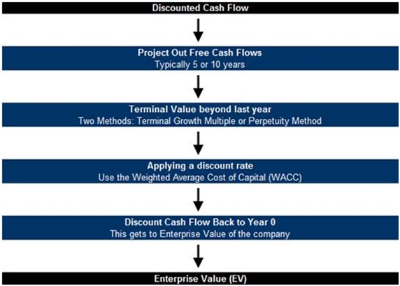
DCF Steps

1. Project the company’s Free Cash Flows: Typically, a target’s FCF is projected out 5 to 10 years in the future. The further these numbers are projected out, the less visibility the forecaster will have (in other words, later projection periods will typically be subject to the most estimation error).
2. Determine the company’s Terminal Value: Terminal Value is calculated using one of two methods: the Terminal Multiple Method or the Perpetuity Method. (Note that if the Perpetuity Method is used, the Discount Rate from the following step will be needed.)
3. Determine the company’s Discount Rate: Calculate the company’s Weighted Average Cost of Capital (WACC) to determine the Discount Rate for all future Cash flows.
4. Use Net Present Value: Discount the projected FCF and Terminal Value back to Year o (i.e., back to today) and sum these figures to determine the Enterprise Value of the company.
5. Make Adjustments: If using an Unlevered Free Cash Flow (UFCF) approach, subtracting out net debt and other adjustments from Enterprise Value to derive the Market Value of the company.

Here is a graphical representation of these DCF Steps:

Sources of DCF Information

In order to project a company’s future Cash flows reasonably well, the analyst will need to take into account as much known information about the company (and several market metrics) as possible. The following sources can help provide needed information to produce a high-quality DCF analysis:

• Historical Financial Results:
  • The SEC (http://www.sec.gov/) has company Annual Reports (10-K), Quarterly Reports (10-Q), and Investment Prospectuses (where available).

 

• Cost of Debt:
  • Use a weighted average of the Debt interest rates in a company’s capital structure to calculate the company’s pre-tax Cost of Debt.
  • This information is almost always available for each Debt instrument in a Company’s Annual Reports (10-K) and Quarterly Reports (10-Q).

 

• Cost of Equity:
  • The Risk Free Rate:
    • The risk-free rate is needed in determining the Cost of Equity, and is estimated as a function of the current long-term Treasury Bond rate (assuming that the company’s cash flows are being projected in terms of US$). The benchmark rate used is generally that of the 10-year bond.
    • The Department of the Treasury (http://www.treasury.gov/) publishes U.S. treasury bond rates on a daily basis.
    • For European companies, use the relevant rate from Euro-denominated government bonds.
  • Beta :
    • Beta is a measure of the relationship between changes in the prices of a company’s securities and changes in the value of an overall market benchmark, such as the S&P 500 index.
    • Bloomberg, FactSet, Google Finance, and Capital IQ all publish historical and estimated Beta figures for individual stocks. If the Beta is not published, it can be estimated by means of a simple linear regression.
  • Market Risk:
    • The Market Risk Premium is a measure of the degree to which investors expect to be compensated for owning risky equity securities, rather than risk-free, fixed-rate investments (such as in government bonds). It is calculated using the Capital Asset Pricing Model, which assumes that the ONLY source of risk that demands compensation is overall market risk (as measured by Beta) rather than idiosyncratic (or stock-specific) risk. This model is generally used to determine the Cost of Equity for a company.
    • Estimates of the Market Risk Premium are available from Morningstar, and can also be estimated using historical returns on government bond investments vs. overall equity market investments.

 

• Financial Projections:
  • Management Estimates can be a useful starting point for determining a company’s expected performance and Cash flow projections. However, keep in mind that these projections are often on the optimistic side.
  • Sell-side Research Estimates also can provide useful insight into a company’s path of expected performance. Again, however, keep in mind that sell-side analysts often have an incentive to be optimistic in projecting a company’s expected performance.
  • Internal Estimates (from the investment bank you work for) can be the most useful source of information for projecting a company’s expected Cash flow—particularly if these estimates were not used as part of a sell-side advisory engagement (wherein the purpose of the analysis would be, at least in part, to advocate for a higher selling price for the client). If using internal estimates, be sure to note how they were generated and for what purpose.

Free Cash Flow (FCF)

In projecting Free Cash Flow for a business, remember “C.V.S.”, and that Garbage In = Garbage Out:

• Confirm historical financials for accuracy.
• Validate key assumptions for projections.
• Sensitize variables driving projections to build a valuation range.

In order to calculate Free Cash Flow projections, you must first collect historical financial results.

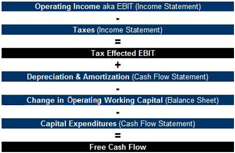
Key Inputs to Free Cash Flow (FCF)

Free Cash Flow (FCF) is calculated by taking the Operating Income (EBIT) for a business, minus its Taxes, plus Depreciation & Amortization, minus the Change in Operating Working Capital, and minus the company’s Capital Expenditures for the year. This derives a much more accurate representation of the Cash that a company generates than does pure Net Income:

Projecting Free Cash Flow (FCF)

 

Key Assumptions in Projecting Business Performance

The projected FCF in the nearest-out years (Year 1, Year 2, etc.) will have the most impact on a company’s DCF valuation. The good news is that these Cash flow figures are the least difficult to project, because the closer we are to an event, the more visibility we have about that event. (The bad news, of course, is that any error in projecting these figures will have a large impact on the output of the analysis.)

FCF is derived by projecting the line items of the Income Statement (and often Balance Sheet) for a company, line by line. As a result, the FCF results are sensitive to a variety of assumptions about the future operations of the company’s business, including the following:

• Income Statement Items:
  • Revenue (Sales) Growth: Year-over-year growth projections are the most common mechanism, but the more granularity used, the better. For example, being able to project out unit growth and pricing per unit is better than a simple year-over-year growth projection for the Sales number as a whole.
  • Margins: Project Gross Margin and Operating (EBIT) Margin based on historical patterns. Consider inputs like commodity costs in Gross Margin and SG&A (Sales, General, and Administrative) expenses for Operating Margin.
• Balance Sheet & Statement of Cash Flow Items:
  • Capital Expenditures (CapEx): Consider both Expansion CapEx and Maintenance CapEx. The difference delineates company costs associated with buying new fixed assets to facilitate growth in the business (Expansion CapEx) from company costs associated with adding to/maintaining the value of existing assets required to service existing business (Maintenance CapEx). Unfortunately, this breakdown is generally unavailable in a company’s financial reports.
  • Changes in Operating Working Capital (OWC): Operating Working Capital is equal to Current Assets minus Current Liabilities, excluding Cash, Cash-like items (such as Marketable Securities and Securities Available for Sale), and Debt. It can be found by incorporating the relevant line items from the Balance Sheet. Use historical patterns and common sense to evaluate this line item—most OWC items are driven by Sales of the company. Thus, growth in these items should at least to some extent be a function of Sales growth.

Remember “C.V.S.” when projecting all of these items. The assumptions driving these projections are critical to the credibility of the output.

• Confirm historical financials for accuracy.
• Validate key assumptions for projections.
• Sensitize variables driving projections to build a valuation range.

 

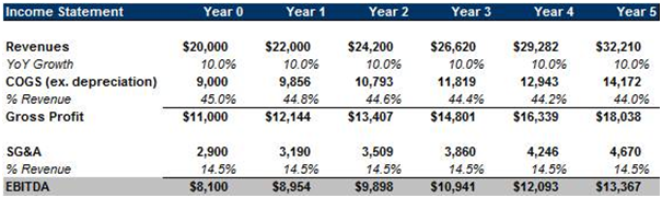
Projecting Business Performance

As mentioned, we first project the company’s Income Statement. Below, we will walk you through a simple example of how to do this.

• Revenue: For simplicity, Revenue in our example is projected out at an annual growth rate of 10%, which is in-line with historical growth rates of the hypothetical company. In order to increase accuracy for this assumption, remember to study management projections, sell-side projections, and internal estimates. Also remember that more granularity, where possible, is better.
• Cost of Goods Sold (COGS): As Revenue grows, we increased the gross profit margin by shrinking COGS as a percentage of Revenue because of the concept of economies of scale at the company (as the company grows it should experience at least some improved utilization of existing equipment and human resources, increased purchasing power, increased pricing power, etc.). Also note that for the purposes of this simple example, we are excluding Depreciation from COGS. In many cases, we would include it and back it out later.
• Selling, General, & Administrative (SG&A): Kept constant as a percentage of Revenue (14.5%) in this example, as the company will need to increase advertising and overhead in order to drive Sales growth. In some cases, some portion of SG&A can be considered fixed (such as Corporate Headquarters costs), which may lead to diminishing SG&A expenses as a percentage of Sales as the company grows.
• EBITDA: This is a direct output of our Revenue and cost assumptions. Had we incorporated Depreciation into expenses, we would need to add it back to Operating Income (EBIT) to arrive at EBITDA.

Depreciation and Capital Expenditures

Depreciation is a non-Cash expense, meaning the company books Depreciation as an expense on the income statement for GAAP (Generally Accepted Accounting Principles) purposes but in reality, no Cash was actually spent. It is an expense of Capital Expenditures made in prior years. Therefore, in order to calculate true “Cash flow,” this must be added this back. Similarly, CapEx must be subtracted out, because it does not appear in the Income Statement, but it is an actual Cash expense.

It should be noted that Amortization acts in much the same way as Depreciation, but is used to expense non-Fixed Assets rather than Fixed Assets. An example of this would be Amortization on the value of a patent purchased when acquiring a company that owned it.

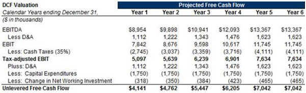
Building up to Unlevered Free Cash Flow

The next step is to take our business performance projections and calculate Unlevered FCF (UFCF) in each year:

• Tax-adjusted EBIT: D&A needs to be taken out of EBITDA in order to calculate after-tax Operating Profit (aka EBIT). D&A is an expense for tax purposes. Thus, first we must subtract D&A in this model to calculate taxes, and then add it back after taxes. In this case, it is projected as 5.1% of Sales.
• Tax Rate: Use last twelve months (LTM, also referred to as trailing twelve months, or TTM) tax rate in order to project future tax rates. In this case, 35% is used.
• Depreciation & Amortization (D&A): D&A was initially taken out to calculate taxes but then added back, because it is a non-cash expense. Capital Expenditures (CapEx): Subtracted out, as this represents Cash needed to fund new and existing assets. It is not expensed on the Income Statement, as these purchased assets will be used to support operations in upcoming years for the business (and is thus gradually expensed, via Depreciation, in those years). Note that net of inflation, CapEx and Depreciation should converge over time, provided that the company is not growing rapidly.
• Change in Operating Working Capital (OWC): This is subtracted out, as it represents investments in short-term net operating assets needed to fund Revenue growth. This figure represents the annual change in Current Assets minus Current Liabilities on the Balance Sheet, excluding Cash, Cash-like items, and Debt.

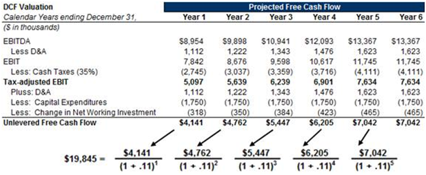
Now we can apply the formula:

Discounting the UFCF Figures

We have now projected the expected Unlevered Free Cash Flows (UFCF) in each of the upcoming years. However, to value the company, we have to discount those cash flows into equivalent current (today’s) dollars. This is where Net Present Value (NPV) comes in.

The formula for calculating Present Value (PV) is as follows:

In this formula, the PV is equal to the FCF in each year (Year 1, Year 2, Year 3, etc.), divided by a discount factor. In each case, the discount factor is 1 + the discount rate (r), taken to the nth power, where n is the number of years into the future that the Cash flow is occurring (similar to the compounding of an annual interest rate).

We will go into more detail on determining the discount rate, r, in the WACC section of this chapter.

The difference between Present Value and Net Present Value is simply to incorporate any cash outflows that might occur in the scenario. Since a DCF analysis involves only the cash inflows from a company’s operations, Present Value and Net Present Value are equivalent.

Terminal Value

Terminal Value represents the value of the cash flows after the projection period. Projections only go out so far in the DCF (i.e. 5 or 10 years), so this is a mechanism for estimating the future value of the business’s cash flows after that projection period.

The Terminal Value is based on the cash flows of the business in a normalized environment. What this means is that the business should be assumed, after the projection period, to grow at a rate that is appropriate for a business of its type at the end of the projection period, and/or to be valued at multiples consistent with those of its peers (see the chapter on Comparable Companies Analysis earlier in this training course).

Calculating Terminal Value

There are two primary methods to compute a company’s terminal value:

1. Terminal Multiple Method: Also referred to as the Exit Multiple Method, this technique uses a multiple of a financial metric (such as EBITDA) to drive a business’s valuation. These multiples can be derived using multiples prevalent among comparable companies.
2. Perpetuity Method: Assumes that the Free Cash Flows of the business grow in perpetuity at a given rate. The Perpetuity Method uses the Gordon Formula: Terminal Value = FCF_n × (1 + g) ÷ (r – g), where r is the discount rate (discussed in the next section on WACC) and g is the assumed annual growth rate for the company’s FCF. This will be demonstrated with an example shortly.

As a sanity check, you can use the terminal method to back into an assumed growth rate for the business, which should be similar to the growth rate used in the perpetuity method. Examples of this calculation are discussed later in this section.

Using the Terminal Multiple Method

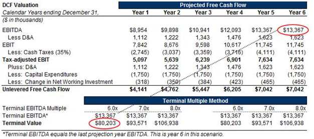
Continuing with our DCF example from earlier, we will demonstrate the two steps needed to apply the Terminal Multiple Method:

1. Identify reasonable EBITDA multiple range. For this exercise, we are assuming a range of 6.0x-8.0x EV/EBITDA. We chose 6.0x to 8.0x based on historical trading ranges for the company along with comparable companies in the industry.
2. Multiply the EV/EBITDA multiple range by the end of period EBITDA estimate. The result equals the Enterprise Value of the company as of the end of the projection period.

Here are a couple of important considerations to make when using the Terminal Multiple Method:

• Make sure the terminal year is a “normalized” year. Exclude years that are influenced cyclical factors or economic factors.
• The growth rate that the EBITDA multiple implies needs to be in-line with long-term assumptions.
• Be sure to use a “normalized” tax rate in the terminal year. A tax rate can be skewed by previous losses, one-time items, and a change in international mix.

 

Using the Perpetuity Method

The Perpetuity Method uses the assumption that the Free Cash Flows grow at a constant rate in perpetuity over the given time period. You should use a conservative approach when estimating growth rates in perpetuity. Analysts typically use long-term growth rates such as GDP growth (or perhaps something slightly higher), as companies typically can’t register double digit FCF growth rates forever.

Here are the two steps needed to apply the Perpetuity Method:

1. Identify reasonable long-term FCF growth rates to use in perpetuity, such a GDP or something slightly higher, depending on industry and company dynamics.
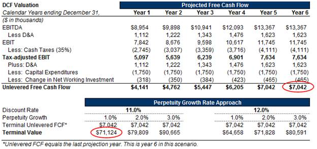
2. Calculate the Terminal Value by taking FCF from the last projection year times (1 + the perpetual growth rate). Divide this figure by the difference between the discount rate (r) and the assumed perpetual growth rate (g).

In this case:

• FCF_n = last projection period Free Cash Flow (Terminal Free Cash Flow)
• g = the perpetual growth rate
• r = the discount rate, a.k.a. the Weighted Average Cost of Capital (WACC, covered in the next section of this training course)

If we assume that WACC = 11% and that the appropriate long-term growth rate is 1%, we get:

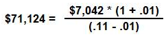
This is a very conservative long-term growth rate, and of course higher assumed growth rates will lead to higher Terminal Value amounts.

Reconciling the Two Methods

Note that there are formulas to determine the equivalent multiples and growth rates for the two given methods.

• Using the Terminal Multiple Method to solve for the equivalent Perpetuity Method growth rate:

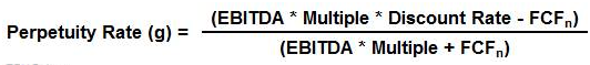
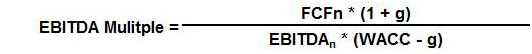
• Using the Perpetuity Method to solve for the equivalent Terminal Multiple Method multiple:

Weighted Average Cost of Capital (WACC): Different ways to describe the same concept

WACC can be a confusing concept. The technical definition of WACC is the required rate of return for the entire business given the risks to investors of investing in the business. Meanwhile, the layperson’s (and probably analyst’s) definition of WACC is the rate used to discount projected Free Cash Flows (FCF) in a DCF model.

These definitions refer to two sides of the same coin. If an investor requires a specific return on his investment dollars today, then future cash flows from an investment he makes can be converted into today’s dollars using that required return to create a “today-equivalent” value for those future cash flows. (The WACC simply does this for all investors in a company, weighted by their relative size.) Since the future FCF represent all of the value of a company available to all investors (Debt and Equity) in the company, they can be discounted by WACC to determine their value in today’s dollars.

But how do we determine what that required return should be? Put simply, it is a function of the alternative investment opportunities available to all of the investors in the company, and the riskiness of making that investment in the company relative to those available alternative returns. If the risk-equivalent return in other opportunities is X% per year, then an investor should require X% from this investment as well. And in order to gauge the current value of the investment in today’s dollars, we need to discount all future benefits accruing to those investors (namely, future Cash flows) by X%.

Here is a summary of things to make sure you understand about the WACC:

• When discounting back projected Free Cash Flows and the Terminal Value in the DCF model, the discount rate used for each Cash flow is WACC.
• The capital structure mix of Debt (tax-affected) and Equity times the Cost of Debt and Cost of Equity equals the WACC. In effect, WACC is the after-tax weighted average of the Costs of Capital for Debt and Equity, where the weights correspond to the relative amount of each component that is outstanding.
• WACC is a forward-looking rate of return and is directly related to the risk of the investment and the alternative investment opportunity set available to the company’s investors across the capital structure (i.e., for the business as a whole, not just for the shareholders).

Now that we have described WACC and what it represents fully, here is the mathematical definition of WACC:

Where:

• K_E = Cost of Equity. K_E = K_rf + b × RP, where K_rf equals the Risk Free Rate, b equals the levered (Equity) Beta for the company, and RP equals the Equity Market Risk Premium. The Beta and Risk Premium are calculated using the Capital Asset Pricing Model (CAPM).
• K_D = Cost of Debt. This is the weighted average of interest rates paid on the company’s debt obligations. Notice that in WACC, Cost of Debt is taken after taxes—i.e., it is multiplied by (1 – T). This is to acknowledge the fact that Interest Expense on Debt is (generally) tax-deductible, thereby creating a tax shield which adds value to the company. This is represented in the DCF framework by reducing the Cost of Debt component of WACC, resulting in a lower discount rate for the company’s FCF, and therefore a higher valuation for the company.
• E = Market Value of Equity, i.e., Market Capitalization.
• D = Book Value of the company’s Debt.
• T = Marginal Tax Rate for the company. This rate can be different from the Effective Tax Rate used to determine Tax Expense based on EBIT.

 

Calculating WACC: An Example

Here is an example that illustrates the calculation of WACC for our hypothetical company, using the average adjusted (levered) beta for a sample of hypothetical, comparable companies:

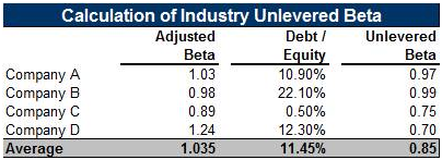
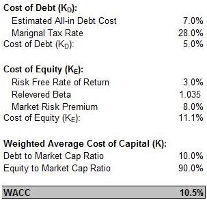
Other WACC Hints:

• WACC takes into account a capital structure that is assumed not to change over time. If it does, and that change is known, the WACC associated with each future capital structure should be used instead. An example of this might be a company in a leveraged buyout (LBO) where the capital structure will be changing as the company reduces Debt.
• When using a DCF analysis to value an M&A transaction, use the target company’s WACC rather than that of the acquiring company. This is because the WACC of the target company will more accurately reflect the relevant risks inherent in the business being acquired.

←Comparable Company AnalysisPrecedent Transaction Analysis→