In this chapter we will introduce the reader to some key, high-level concepts required to understand valuation and how it’s done on Wall Street. We will cover three key topics:

• Enterprise Value: The 30,000-Foot View
• Understanding Enterprise Value vs. Market Value
• An Introduction to Valuation Techniques

Enterprise Value: The 30,000-Foot View

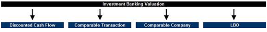
Investment bankers use four primary valuation techniques when advising corporate clients. These techniques apply almost universally, regardless of the company, industry or circumstance. They will be introduced in the next chapter, Valuation Techniques Overview.

But how are the valuation techniques actually constructed? When should which technique be used? What are the basic building blocks required for them? We will find more detailed answers to some of these questions in the next chapter. However first we’re going to take a step back and explain some of the building blocks of these valuation techniques so that they make sense when we later discuss them in technical depth.

In this chapter, therefore, you will find a detailed overview of the core building blocks of the valuation techniques used by investment bankers.

Enterprise Value (frequently referred to as EV—not to be confused with Equity Value, which is another name for Market Value of a company) is the core building block used in financial modeling. The reason is this: Enterprise Value is designed to represent the entire value of the company’s operations. By contrast, Market Value is a residual: it represents the value of the company remaining once the value ascribed to other stakeholders (non-owners) has been taken out.

Enterprise Value must therefore account for all of the differences between Market Value (remember, this figure is the Market Value of a company’s Equity or ownership) and the Value of Operations (or Operating Value) of a Company.

Let’s start with a basic identity equation:

This equation is simple enough. Assuming that the company is profitable, and that it’s more valuable in operation than in liquidation (in other words, the company is worth more money if it continues in business rather than stopping business and selling off the assets to the highest bidders), the value of the company is equal to the value of its productive operations. This value must also equal the value of all of the net claims against the company’s assets, because these assets are being used to produce money for these claimants, or stakeholders (assuming, of course, that these claims have been valued correctly). The “Excluding Excess Cash” piece will be explained in a moment.

The net value of all the claims on a company’s assets can be broken down as follows:

• Debt: Money that has been lent to the company by another person or institution. Debt holders have a higher priority than equity holders on the claims of the company’s assets and value, so they get paid first. In order to get to EV, we must add Debt to the Market Value of the company’s Equity.
• Cash: Money that is owned by the company—in other words, it’s sitting on the company’s balance sheet. This money, assuming it is not required by the operations of the business, could be used to pay off existing claimants, or stakeholders. (For example, the cash could be used to pay off Debt; it could also be used to repurchase outstanding shares in the company’s Equity.) Thus the higher the Cash balance a company has, the less its operations must be worth. This concept is counterintuitive: shouldn’t owning more cash be a good thing? Yes, in a sense it is—but assume for a moment that a company’s Market Value (of Equity) is fixed at a certain dollar amount. That value can be ascribed to only two sources: (1) the residual claim value on a company’s operations after all other stakeholders have been paid off, and (2) the value of the money on the company’s balance sheet. The higher (2) is, the lower (1) is, and vice versa. Therefore, to get to EV, we must subtract Cash from the Market Value of the company’s Equity. (This is one way of looking at it. In practice, Cash is often subtracted from Debt to get an important statistic called Net Debt. Net Debt is the value of the Debt once balance sheet Cash has, hypothetically, been used to pay some of it off. Diagrams below will explain the different ways of conceptualizing this.)
• Minority Interest: This is a tricky one. Corporations often have a Liability account called Minority Interest (MI). This is a special accounting designation for a specific scenario: when a Corporation owns most, but not all, of a subsidiary company. If that is the case, the subsidiary company is consolidated entirely into the Corporation’s financial statements, so that it would appear, at first glance, that the Corporation does indeed own 100% of that subsidiary. In fact it does not, so this Liability account is created to represent the value of the shares owned in the subsidiary by other individuals or companies. (Similarly, there will be a corresponding Minority Interest expense on the Income Statement for the Corporation, representing the portion of value from the subsidiary’s operating results that actually belongs to the other shareholders in the subsidiary.) Since this MI represents the value of the partial ownership (by others) in this subsidiary, it should be treated like Debt – that is, in order to get to EV, we must add Minority Interest to the Market Value of the company’s Equity. (We should keep in mind, then, that this EV statistic will include the entire value of the company’s subsidiary, even though the Corporation itself does not own 100% of it.)
• Preferred Equity: Despite the name, Preferred Equity primarily operates as Debt, not Equity. It is junior to all other forms of Debt, but it is also senior to the Equity (often called Common Equity or just “common.”) Often, Preferred Equity can be converted to shares of Common Equity, hence the name. It may be convertible to Common Equity but, until that time, it receives interest and is in line ahead of the Common Equity in the capital structure, so it is “preferred” to the common shares. It receives preferential treatment. Because Preferred Equity is actually primarily Debt unless and until it is converted to Equity, we must add Preferred Equity to the Market Value of the company’s (Common) Equity.

Visually, we can look at this two different ways:

1. Enterprise Value + Cash = Total Value of All Claims

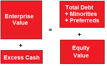
2. Enterprise Value = Net Value of All Claims

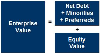
Typically, investment bankers and investors look at this equation the second way (the Net Debt/Net Value version). This is the one to be most familiar with.

Another View of Enterprise Value

There is another way of looking at EV: core assets vs. non-core assets. Core assets are used to generate profit for the business; non-core assets are things owned by the business but not central to its money-generating operations.

• Core Assets: assets critical to the operating business, such as Inventory, Fixed Assets, Accounts Receivable, etc.
• Non-Core Assets: assets not critical to the operating business such as Derivatives, Currencies, Real Estate, Commodities, Stock Options, etc.

In this sense, Cash on the Balance Sheet usually (at least for the most part) is non-core. Unless it’s cash that the business needs to operate (such as dollar bills in the registers at a retail operations), it is not being used to generate profit in the business operations. That’s why it is stripped out in EV calculations. (Other non-core assets may be as well, especially if they can be sold off for cash without harming the operations of the business. For example, Real Estate and Commodities can often be sold without impacting the Company’s cash-generating operations.)

Therefore Cash is (generally) a non-core asset. Other similar assets, such as Marketable Securities, are simply ways of attempting to earn profit on that Cash, but are not core to the company’s operations. These Cash-like assets can also be sold off, and should be stripped out of the Net Debt Calculation.

Primary Components of Net Debt

• (+) Short-Term Debt: Debt with less than one year maturity.
• (+) Long-Term Debt: Debt with more than one year maturity.
• (+) Debt Equivalents: Operating Leases and Pension Shortfalls.
• (–) Cash and Cash Equivalents: Cash, Money Market Securities, and Investment Securities

Notice in this list that “Cash and Cash Equivalents” is a subtraction from the calculation—Cash and Cash-like assets are thus a sort of “anti-Debt.” Debt can also come in several different flavors, but on the Balance Sheet it’s almost always broken down into Short-Term Debt and Long-Term Debt. This is because Short-Term Debt is coming due soon (within less than a year), and thus must be paid off or refinanced in the near future. This may be of interest if the company is having financial trouble—the due date on the near-term Debt may trigger difficulties for the Company in terms of repayment. This type of difficulty, which can end up being a crisis under the right circumstances, is called a liquidity problem (or crisis).

Understanding Enterprise Value vs. Market Value

Nearly all valuation techniques will focus on either Enterprise Value or Market Value (or Equity). So which do we use, and when? In a nutshell:

Let’s start by looking at three commonly used trading multiples:

• EV/Sales: Enterprise Value ÷ Sales (or Revenue)
• EV/EBITDA: Enterprise Value ÷ EBITDA (Earnings before Interest, Taxes, Depreciation & Amortization)
• Price/Earnings (or P/E): Market Value of Equity ÷ Net Income (alternatively, Stock Price ÷ Earnings Per Share, or EPS)

Notice that in the first two examples, Enterprise Value is used. This is because Sales and EBITDA generate profit/value that is available to all stakeholders. No compensation has yet been taken out for non-Equity stakeholders. By contrast, Price/Earnings reflects the Net Income for a company, which is computed after compensation for other stakeholders has been removed (Interest Expense and Minority Interest). Therefore, this profit/value is only available to Equity stakeholders.

People new to valuation may ask, “Why is it incorrect to use Market Value/EBITDA or Enterprise Value/Net Income?” The answer lies in the fact that for any multiple, the denominator and numerator within that multiple must either include or exclude leverage. In other words, both the numerator and denominator must both relate to either all stakeholders or only shareholders. Otherwise, comparisons across companies will not be “apples-to-apples”—they will be difficult to compare because different companies utilize different amounts of leverage.

This concept is demonstrated in the following graphic:

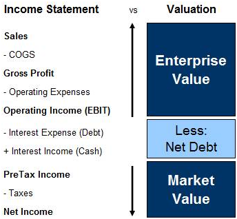
In summary:

An Introduction to Valuation Techniques

You will read about the four main valuation techniques for Investment Bankers in great detail in the upcoming chapters. Here is a brief overview of them all, with this concept of Enterprise Value vs. Market Value in mind:

Comparable Company Analysis

• Comparable Company Analysis, frequently referred to simply as “Comps,” is a valuation technique used to find company values based on traded values of similar (comparable) companies.
• Comps a market-based valuation analysis relying on current market prices for publicly traded companies.
• Comps valuation can revolve around either the Enterprise Value of the company or the Market Value of the company, depending on the multiples being used. For example, EV/Sales or EV/EBITDA multiples would refer to Enterprise Value, while Price/Earnings multiples (equivalent to Market Value/Net Income) would refer to Market Value.

The Three Main Steps of a Comps Valuation

1. Identify publicly-traded companies with characteristics similar to those of the company being valued.
2. “Spread” the Comps—i.e., map-out the trading multiples (EV/Sales, EV/EBITDA, and P/E) for this set of comparable companies.
3. Assign these multiples to company financial results to determine valuation ranges.

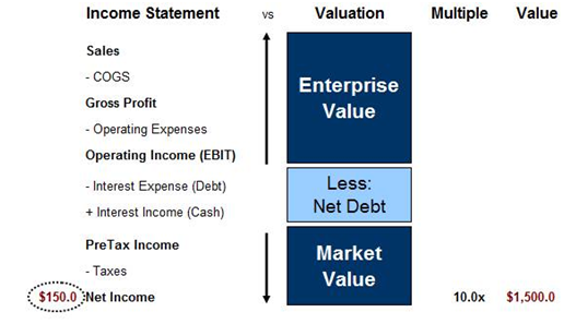
Comparable Companies Analysis Example

• ABC Company is currently generating annual Net Income of $150 million.
• Publicly traded comparable companies are trading, on average, at 10x current year Net Income.
• How much is the Equity of this company worth?

Using Comparable Company Analysis, this company’s Equity is worth $1.5 billion based on $150 million of Net Income and the comparable company average of 10x Net Income. Note that a proper range of the valuation can be obtained by looking at the highest and lowest Net Income multiples in the comparable companies set.

Discounted Cash Flow (DCF) Analysis

• DCF analysis values a company by projecting its future Free Cash Flows (FCF) and then using the Net Present Value (NPV) method to value the firm.
• DCF valuation builds off of Free Cash Flow forecasts that are typically done for the upcoming 5 to 10 years.
• DCF valuation primarily returns the Enterprise Value of the company, because Free Cash Flow refers to the cash generated by the operations of a business, irrespective of Net Debt and Minority Interest/Preferred Equity. However a DCF model can also be used to project Market Value if Interest Expense and Minority Interest are projected and stripped out to produce Levered Free Cash Flows (LFCF).

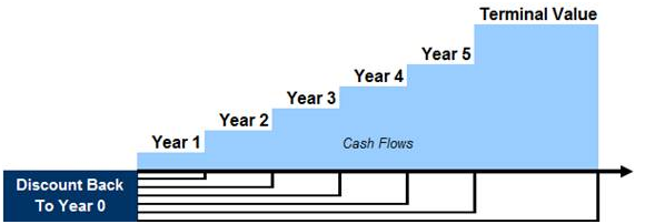
The Four Main Steps of a DCF Valuation

1. Forecast out a company’s Free Cash Flows for the next 5-10 years.
2. Calculate the Weighted Average Cost of Capital (WACC).
3. Calculate the firm’s Terminal Value, or the future value of the firm assuming a stable long-term growth rate.
4. Discount 5-year Free Cash Flows plus Terminal Value back to Year 0 (today) to derive the Enterprise Value of the company.

Free Cash Flows are discounted back to Year 0 (today) to solve for Enterprise Value, as displayed in this graphic:

Precedent Transaction Analysis

• Precedent Transaction Analysis, also called “Comparable Transactions,” looks at recent historical M&A activity involving similar companies to get a range of valuation multiples.
• This transaction valuation analysis relies on whatever historical M&A transaction information is available.
• Precedent Transaction valuation can revolve around either the Enterprise Value of the company or the Market Value of the company, depending on the multiples being used. For example, EV/Sales or EV/EBITDA multiples would refer to Enterprise Value, while Price/Earnings multiples (equivalent to Market Value/Net Income) would refer to Market Value. The most commonly used transaction multiples are EV/Sales, EV/EBITDA, and P/E.

The Three Main Steps of Precedent Valuation

1. Identify publicly traded companies with similar characteristics.
2. “Spread” the comps or map-out trading multiples such as EV/Sales, EV/EBITDA, and P/E.
3. Assign industry multiples to company figures to determine valuation ranges.

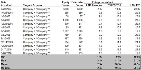
Precedent Transaction Analysis Example

• PDQ Company is currently generating annual Net Income of $150 million.
• Precedent M&A transactions since 2004 have shown industry average of 20x P/E (see image below).
• How much is the Equity of this company worth?

Using Precedent Transaction Analysis, PDQ’s Equity is worth $3.0 billion based on $150 million of Net Income and the precedent P/E multiple of 20x Net Income. Note that a proper range of the valuation can be obtained by looking at the highest and lowest Net Income multiples in the precedent transactions set.

Leveraged Buyout (LBO) Analysis

• An LBO is the acquisition of a public or private company with a significant amount of borrowed funds. Leveraged Buyout Analysis is discussed later in this training module; it is also discussed in great depth in the Private Equity Training Module.
• LBO acquirers are typically Private Equity sponsors.
• This is a transaction-based valuation technique. Private Equity buyers typically look to sell the business within 5 years after purchase.
• LBO valuation revolves around the Enterprise Value of the company, because the entire business will be acquired and all (or essentially all) of the pre-existing Debt will be paid off.

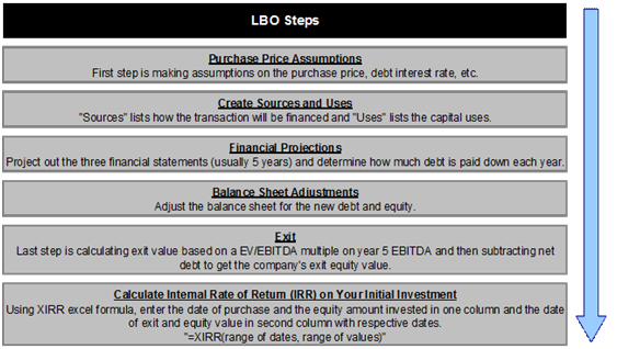
The Five Main Steps in an LBO Analysis

1. Make transaction assumptions based on the purchase price, Debt interest rate, etc.
2. Build the Sources & Uses table, where “Sources” lists how the transaction will be financed and “Uses” lists the capital uses—i.e., where the “Sources” money will be spent.
3. Adjust the Balance Sheet for the new Debt and Equity, and other transaction-related adjustments.
4. Project out the three financial statements (usually 5 years) and determine how much Debt is paid down each year.
5. Calculate exit value scenarios based on EBITDA multiples.

←IntroductionValuation Techniques Overview→